Day 1 Notebook Intro
Initial Setup of Python Environment
Over the course of the next few days, we will rely on a number of python modules. Google Colaboratory comes equipped with a large number of these modules, but there are a few that we need that are not provided by default. Run the cells below to install these modules. You can optionally comment out modules that are only necessary for specific days that you will not be attending.
# Get non-default modules
!pip install rdkit-pypi
Activity 1: Concepts with Linear Regression
Many of the important concepts in supervised machine learning can be appreciated by a solid understanding of linear regression, which we all probably encountered early on – like elementary school. We are going to work through a linear regression task in a fashion to appreciate many of the basic mechanics that underlie deep learning.
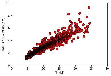
To start, we will pull a dataset generated in a recent paper that explores the use of machine learning to predict polymer properties. The label that we extract (and our target for prediction) will be the radius of gyration (\(R_g\)), which provides a measure of an object’s size, for some simulated intrinsically disordered proteins.
A well known result from polymer physics is that \(R_g \propto M^{0.5}\), where \(M\) is the number of some statistically uncorrelated sub-units in the polymer; the same result arises in the context of diffusion/random walks.
In the following, we will examine how well the data on \(R_g\) can be described by a simple linear model with \(N^{0.5}\) as our input feature (\(N\) will be the number of residues in the protein, which we do not generally expect to be a statistically uncorrelated sub-unit)
Run the cell below to obtain and view the data.
# modules for this activity
import pandas as pd
import matplotlib.pyplot as plt
import numpy as np
from sklearn.metrics     import r2_score, mean_squared_error,mean_absolute_error
from sklearn.model_selection  import train_test_split, KFold
def plot_raw_data(x,y):
  plt.plot(x, y,marker='o',linestyle="",markersize=8,color='r',markeredgecolor='k')
  plt.ylabel("Radius of Gyration (nm)")
  plt.xlabel("N^0.5")
  plt.xlim(0,30)
  plt.ylim(0,10)
  return plt.gca()

url_for_labels    = "https://raw.githubusercontent.com/webbtheosim/featurization/main/Dataset_A/labels.csv"
url_for_sequences = "https://raw.githubusercontent.com/webbtheosim/featurization/main/Dataset_A/sequences.txt"
idpdata = pd.read_csv(
    url_for_labels
)
idpdata.head()
y = idpdata['ROG (A)'].to_numpy()/10.     # these are now labels

import urllib.request
import random

seqs  = [line.strip().split() for line in urllib.request.urlopen(url_for_sequences)]
X     = np.array([len(seq) for seq in seqs])**0.5   # these are features

ax = plot_raw_data(X,y)
Examining a human hypothesis
At first glance, it certainly seems that there is reasonable linear correlation between our input and labels.
We are going to consider a function of the form
Can you look at the plot to “guess” values of these parameters? Complete the cell below and explore some “hypotheses”.
# basic set up
Nmax = 900
xline= np.array(range(Nmax+1))**0.5
f    = lambda x, th: th[0] + th[1]*x

#$$$$$$$$$$$$$$$$$$$$$$$$$$$$$$$$$$$$$$$$$$$$$$$$$$$$$$$$$$
# fill in parameters
thetas = np.array([[VALUE1,VALUE2]]).T # this maps to a 2x1
#$$$$$$$$$$$$$$$$$$$$$$$$$$$$$$$$$$$$$$$$$$$$$$$$$$$$$$$$$$

# make predictions using function
yline = f(xline,thetas)

# examine hypothesis
ax = plot_raw_data(X,y)
ax.plot(xline,yline,color='y',linewidth=3,linestyle=':')
plt.show()

# make predictions from features and compute evaluation metrics
yhat  = f(X,thetas)
r2    = r2_score(y,yhat)
rmse  = mean_squared_error(y,yhat)
mae   = mean_absolute_error(y,yhat)
print("r2 = {:>5.3f}, MSE = {:>5.3f}, MAE = {:>5.3f}"\
      .format(r2,rmse,mae))
More formal optimization
Probably your human-intuited fit yields a pretty darn good description of the data, but we’ll try to do better.
The ``training’’ of neural networks is really about optimization where the objective is to minimze a loss function that describes a disparity between the model predictions and the ground truth of some set of labels.
When we first encounter linear regression, our optimization is usually in the `least-squares’ sense; that is, our loss function is the mean-squared error over our observations. The problem of linear least-squares regression can be ``exactly’’ solved using techniques from linear algebra, but that is not so much the domain of machine learning. Therefore, we will approach a solution using gradient descent optimization, which is more akin to what is needed fro training a neural network.
Below we define and examine our loss function (a mean-squared error) over our parameter space (considering the whole dataset). We also place a star at the position of the hypothesis that we generated in the previous cell. Is it close to the minimum?
def loss(x,y,theta):
  ''' Function to calculate cost function assuming a hypothesis of form y^ = X*theta
  Inputs:
  x = array of dependent variable
  y = array of training examples
  theta = array of parameters for hypothesis

  Returns:
  E = cost function
  '''
  n        = len(y) #number of training examples
  features = np.ones((n,len(theta))) # X
  features[:,1] = x[:]
  ypred = features@theta # predictions with current hypothesis
  E = np.sum((ypred[:,0]-y[:])**2)/n #Cost function
  return E

def plot_loss(t0,t1,E):
  t0g,t1g = np.meshgrid(t0,t1)
  fig = plt.figure(figsize=(15,4))
  ax1  = fig.add_subplot(1,2,1,projection='3d')
  surf = ax1.plot_surface(t0g, t1g, E, linewidth=0, antialiased=False,cmap='coolwarm')
  ax1.set_xlabel(r"$\theta_1$")
  ax1.set_ylabel(r"$\theta_0$")
  ax1.set_zlabel(r"$E$")
  ax2 = fig.add_subplot(1,2,2)
  CS = ax2.contour(t0g,t1g,E.T,np.logspace(-3,2,25),cmap='coolwarm')
  ax2.set_xlabel(r"$\theta_0$")
  ax2.set_ylabel(r"$\theta_1$")

  return fig,ax1,ax2

#$$$$$$$$$$$$$$$$$$$$$$$$$$$$$$$$$$$$$$$$$$$$$$$$$$$$$$$$$$
#Define grid over which to calculate J
N = 50
theta0Rng = [AAA,BBB]
theta1Rng = [CCC,DDD]
theta0s = np.linspace(theta0Rng[0],theta0Rng[1],N)
theta1s = np.linspace(theta1Rng[0],theta1Rng[1],N)
#$$$$$$$$$$$$$$$$$$$$$$$$$$$$$$$$$$$$$$$$$$$$$$$$$$$$$$$$$$


#Initialize E as a matrix to store cost function values
E = np.zeros((N,N))

# Populate matrix
for i,theta0 in enumerate(theta0s):
  for j,theta1 in enumerate(theta1s):
    theta_ij = np.array([[theta0,theta1]]).T
    E[i,j]   = loss(X,y,theta_ij)

fig,ax1,ax2 = plot_loss(theta0s,theta1s,E)
ax2.plot(thetas[0],thetas[1],marker='*',color='m',markersize=20)
plt.show()
Gradient Descent
Next, we will implement gradient descent to find an optimal set of parameters. For this type of linear model, it is possible to obtain the requisite derivative of the loss function with respect to the parameters analytically. I have used that solution below.
def E2loss(yhat,y):
    return np.sum((np.squeeze(yhat)[:]-y[:])**2)/len(y)

def Grad_Descent(x,y,theta,alpha,nIters,x_te=None,y_te=None):
  '''Gradient descent algorithm
  Inputs:
  x = dependent variable
  y = training data
  theta = parameters
  alpha = learning rate
  iters = number of iterations
  Output:
  theta = final parameters
  E = array of cost as a function of iterations
  '''
  n        = len(y) #number of training examples
  features = np.ones((n,len(theta)))
  features[:,1] = x[:]
  yhat  = features@theta # predictions with current hypothesis
  E_hist = [E2loss(yhat,y)]

  if x_te is not None:
    E_hist_te = [E2loss(f(x_te,theta),y_te)]

  for i in range(nIters):
    e     = yhat[:,0] - y[:]
    theta = theta - (alpha*e[:,np.newaxis].T@features).T #
    yhat = features@theta # predictions with current hypothesis
    E_hist.append(E2loss(yhat,y))
    if x_te is not None:
      E_hist_te.append(E2loss(f(x_te,theta),y_te))

  if x_te is not None:
    return theta,E_hist,E_hist_te
  else:
    return theta,E_hist
Next, we’ll actually run the gradient descent code for a specified number of iterations and observe the outcome. We are also specifying a value of a ``learning’’ rate, which is a so-called hyperparmeter in our model training/optimization.
th0     = np.array([[-1.],[.75]])
nIters = 5000
thetaGD, EGD = Grad_Descent(X,y,th0,8e-6,nIters)
print("theta_0 = {:>8.4f}".format(thetaGD[0,0]))
print("theta_1 = {:>8.4f}".format(thetaGD[1,0]))

fig,ax = plt.subplots()
ax.plot(np.array(range(nIters+1))+1,np.array(EGD),linestyle='-',color = 'k',linewidth=3)
plt.xscale("log")
plt.yscale("log")
ax.set_xlabel("Iterations")
ax.set_ylabel("Loss")
plt.show()

# examine solution
ax = plot_raw_data(X,y)
ax.plot(xline,f(xline,thetaGD),color='k',linewidth=3,linestyle=':')
plt.show()
r2    = r2_score(y,yhat)
mse  = mean_squared_error(y,yhat)
mae   = mean_absolute_error(y,yhat)
print("r2 = {:>5.3f}, MSE = {:>8.5f}, MAE = {:>5.3f}"\
      .format(r2,rmse,mae))
theta_0 =  -0.0384
theta_1 =   0.2827
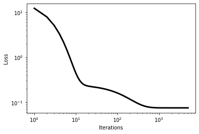

r2 = 0.930, MSE = 0.08822, MAE = 0.162
Linear algebraic solution
If run for enough iterations, the solution obtained from gradient descent should outperform our human-intuited estimated model, even if just slightly. Because this is least-squares linear regression, we can also compare our solution with that obtained via linear algebra.
N = len(y)
M = 2
A = np.ones((N,M))
A[:,1] = X[:]
thetaOpt = np.linalg.inv(A.T@A)@A.T@y
#thetOpt  = np.linalg.pinv(A)@y
yhat  = f(X,thetaOpt)
r2    = r2_score(y,yhat)
mse   = mean_squared_error(y,yhat)
mae   = mean_absolute_error(y,yhat)
print("theta_0 = {:>8.4f}".format(thetaOpt[0]))
print("theta_1 = {:>8.4f}".format(thetaOpt[1]))
print("r2 = {:>5.3f}, MSE = {:>8.5f}, MAE = {:>5.3f}"\
      .format(r2,rmse,mae))
theta_0 =  -0.0384
theta_1 =   0.2827
r2 = 0.941, MSE =  0.08822, MAE = 0.152
Using train/test splits
In our example so far, we did something, which is not generally good practice in machine learning: the data we used to train/optimize the model was the same data that we ultimately tested on. Because of the simplicity of the model that we have here, we are not at significant risk of overfitting, but it is better if we can assess the model using data that was held-out or unseen during training.
In the following cells, we will demonstrate the use of some convenient functions from scikit-learn that allow us to create a simple train/test split of our data.
# create train vs. test split
#$$$$$$$$$$$$$$$$$$$$$$$$$$$$$$$$$$$$$$$$$$$$$$$$$$$$$$$$$$
# write code to use the function train_test_split in scikit learn
# examine the shape of the output arrays and see how they compare
# to the original data structures X and y
# you will want to name the variables as follows
# X_tr --> features for training data
# y_tr --> labels for training data
# X_te --> features for test data
# y_te --> labels for test data


#$$$$$$$$$$$$$$$$$$$$$$$$$$$$$$$$$$$$$$$$$$$$$$$$$$$$$$$$$$


thetaGD, E_tr, E_te = Grad_Descent(X_tr,y_tr,th0,8e-6,nIters,X_te,y_te)
print("theta_0 = {:>8.4f}".format(thetaGD[0,0]))
print("theta_1 = {:>8.4f}".format(thetaGD[1,0]))

fig,ax = plt.subplots()
ax.plot(np.array(range(nIters+1))+1,np.array(E_tr),linestyle='-',color = 'k',linewidth=3)
ax.plot(np.array(range(nIters+1))+1,np.array(E_te),linestyle=':',color = 'r',linewidth=3)
plt.xscale("log")
plt.yscale("log")
ax.set_xlabel("Iterations")
ax.set_ylabel("Loss")
plt.show()

# examine solution
ax = plot_raw_data(X_te,y_te)
ax.plot(xline,f(xline,thetaGD),color='k',linewidth=3,linestyle=':')
plt.show()
yhat = f(X_te,thetaGD)
r2    = r2_score(y_te,yhat)
mse  = mean_squared_error(y_te,yhat)
mae   = mean_absolute_error(y_te,yhat)
print("r2 = {:>5.3f}, MSE = {:>8.5f}, MAE = {:>5.3f}"\
      .format(r2,rmse,mae))
Cross-validation
An important consideration is how the choices that we make when constructing a model impact the model. Some of these choice may include things like hyperparameters associated with training (e.g., the number of training iterations and learning rate) or the actual constitution of our training data. If possible, we would like to mitigate any biases or deficiencies that we introduce in this fashion. Cross-validation provides one framework that can facililitate robustness with respect to the model training and our reporting of its results.
In the next cells, we will perform \(k\)-fold cross-validation to provide a better estimate of prospective model performance.
# We will estimate the model accuracy using cross-validation
k     = 10
kf    = KFold(n_splits=k,shuffle=True,random_state=1)
r2s   = np.zeros([k])
mses  = np.zeros([k])
maes  = np.zeros([k])

for i,(iTrain,iTest) in enumerate(kf.split(y)):
    Xi_tr = X[iTrain]
    Xi_te = X[iTest]
    yi_tr = y[iTrain]
    yi_te = y[iTest]
    thetaGD, E_tr, E_te = Grad_Descent(Xi_tr,yi_tr,th0,8e-6,nIters,Xi_te,yi_te)
    yhat = f(Xi_te,thetaGD)
    (r2s[i],mses[i],maes[i]) = \
    (r2_score(yi_te,yhat),mean_squared_error(yi_te,yhat),mean_absolute_error(yi_te,yhat))

invsqrtk = 1./k**0.5
print("r2 = {:>5.3f} +/- {:>5.3f}".format(np.mean(r2s),np.std(r2s,ddof=1)*invsqrtk))
print("mae= {:>5.3f} +/- {:>5.3f}".format(np.mean(mses),np.std(mses,ddof=1)*invsqrtk))
print("mse= {:>5.3f} +/- {:>5.3f}".format(np.mean(maes),np.std(maes,ddof=1)*invsqrtk))
r2 = 0.941 +/- 0.003
mae= 0.075 +/- 0.006
mse= 0.152 +/- 0.004
import pandas as pd
import rdkit, rdkit.Chem, rdkit.Chem.Draw
from rdkit.Chem.Draw import IPythonConsole
np.random.seed(0)
import warnings
import seaborn as sns
import matplotlib as mpl
IPythonConsole.ipython_useSVG = True
warnings.filterwarnings("ignore")
sns.set_context("notebook")
Activity 2: Chemical Data Basics
In this activity, we will be working with a dataset on the aqueous solubility of various molecules. Our main objective will be to construct and assess the performance of simple linear model for predicting solubility. Although linear modeling is not canonically machine learning, all the concepts and approaches we consider for treating/examining the data as well as evaluating the models will be transferable to building models based on deep learning algorithms.
Execute the following cell to import necessary modules and load the dataset. The data will be loaded into a Pandas dataframe named soldata. After, you can progress through the tasks as described.
# Load the data from dmol-book
soldata = pd.read_csv(
    "https://github.com/whitead/dmol-book/raw/master/data/curated-solubility-dataset.csv"
)
soldata.head()
| ID | Name | InChI | InChIKey | SMILES | Solubility | SD | Ocurrences | Group | MolWt | ... | NumRotatableBonds | NumValenceElectrons | NumAromaticRings | NumSaturatedRings | NumAliphaticRings | RingCount | TPSA | LabuteASA | BalabanJ | BertzCT | |
|---|---|---|---|---|---|---|---|---|---|---|---|---|---|---|---|---|---|---|---|---|---|
| 0 | A-3 | N,N,N-trimethyloctadecan-1-aminium bromide | InChI=1S/C21H46N.BrH/c1-5-6-7-8-9-10-11-12-13-... | SZEMGTQCPRNXEG-UHFFFAOYSA-M | [Br-].CCCCCCCCCCCCCCCCCC[N+](C)(C)C | -3.616127 | 0.0 | 1 | G1 | 392.510 | ... | 17.0 | 142.0 | 0.0 | 0.0 | 0.0 | 0.0 | 0.00 | 158.520601 | 0.000000e+00 | 210.377334 |
| 1 | A-4 | Benzo[cd]indol-2(1H)-one | InChI=1S/C11H7NO/c13-11-8-5-1-3-7-4-2-6-9(12-1... | GPYLCFQEKPUWLD-UHFFFAOYSA-N | O=C1Nc2cccc3cccc1c23 | -3.254767 | 0.0 | 1 | G1 | 169.183 | ... | 0.0 | 62.0 | 2.0 | 0.0 | 1.0 | 3.0 | 29.10 | 75.183563 | 2.582996e+00 | 511.229248 |
| 2 | A-5 | 4-chlorobenzaldehyde | InChI=1S/C7H5ClO/c8-7-3-1-6(5-9)2-4-7/h1-5H | AVPYQKSLYISFPO-UHFFFAOYSA-N | Clc1ccc(C=O)cc1 | -2.177078 | 0.0 | 1 | G1 | 140.569 | ... | 1.0 | 46.0 | 1.0 | 0.0 | 0.0 | 1.0 | 17.07 | 58.261134 | 3.009782e+00 | 202.661065 |
| 3 | A-8 | zinc bis[2-hydroxy-3,5-bis(1-phenylethyl)benzo... | InChI=1S/2C23H22O3.Zn/c2*1-15(17-9-5-3-6-10-17... | XTUPUYCJWKHGSW-UHFFFAOYSA-L | [Zn++].CC(c1ccccc1)c2cc(C(C)c3ccccc3)c(O)c(c2)... | -3.924409 | 0.0 | 1 | G1 | 756.226 | ... | 10.0 | 264.0 | 6.0 | 0.0 | 0.0 | 6.0 | 120.72 | 323.755434 | 2.322963e-07 | 1964.648666 |
| 4 | A-9 | 4-({4-[bis(oxiran-2-ylmethyl)amino]phenyl}meth... | InChI=1S/C25H30N2O4/c1-5-20(26(10-22-14-28-22)... | FAUAZXVRLVIARB-UHFFFAOYSA-N | C1OC1CN(CC2CO2)c3ccc(Cc4ccc(cc4)N(CC5CO5)CC6CO... | -4.662065 | 0.0 | 1 | G1 | 422.525 | ... | 12.0 | 164.0 | 2.0 | 4.0 | 4.0 | 6.0 | 56.60 | 183.183268 | 1.084427e+00 | 769.899934 |
5 rows × 26 columns
Dataset Exploration
One of the first things you should do for any ML task is simply get a feel for the data. As an end goal, we know we want to predict solubility. Thus, solubility is our label for a regression task, and we will try model this as a function of molecular descriptors of a molecule; these are used to construct prospective input feature vectors that represent the molecule.
Summary of Tasks
A. Take a moment to familiarize yourself with the modules that are imported in the previous cell. Then, look at the organization of the DataFrame, the first lines of which are shown above.
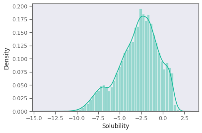
B. Plot the distribution of solubility values. Is there anything notable about its shape or range?
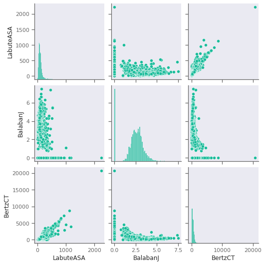
C. Examine pair correlations amongst possible input features. Are any descriptors highly correlated? How do the scale of the features compare?
What does the data look like?
Plot the distribution of solubility values. Is there anything notable about its shape or range?
Useful function: Useful function: sns.distplot https://seaborn.pydata.org/generated/seaborn.distplot.html
#$$$$$$$$$$$$$$$$$$$$$$$$$$$$$$$$$$$$$$$$$$$$$$$$$$$$$$$$$$


#$$$$$$$$$$$$$$$$$$$$$$$$$$$$$$$$$$$$$$$$$$$$$$$$$$$$$$$$$$
plt.show()
Examine pair correlations amongst possible input features. Are any descriptors highly correlated? How do the scale of the features compare? What about correlation with the Solubility?
Useful function: sns.pairplot https://seaborn.pydata.org/generated/seaborn.pairplot.html
Note that if you run pairplot over all features, it may take awhile to run. You may wish to only examine a subset for this reason.
features_start_at = list(soldata.columns).index("MolWt")
feature_names = soldata.columns[features_start_at:]

# code for pair correlations
#$$$$$$$$$$$$$$$$$$$$$$$$$$$$$$$$$$$$$$$$$$$$$$$$$$$$$$$$$$

#$$$$$$$$$$$$$$$$$$$$$$$$$$$$$$$$$$$$$$$$$$$$$$$$$$$$$$$$$$
plt.show()
# code for looking at pair correlations with Solubility
num_cols = 3
num_rows = int( np.ceil(len(feature_names)/ num_cols))
fig, axs = plt.subplots(nrows=num_rows,ncols=num_cols,sharey=True,figsize=(12,12))
axs = axs.flatten()
for i,n in enumerate(feature_names):
  ax = axs[i]
  ax.scatter(soldata[n], soldata.Solubility, s=6, alpha=0.4)
  if i % num_cols == 0:
    ax.set_ylabel("Solubility")
  ax.set_xlabel(n)
  plt.tight_layout()
plt.show()
Feature scaling
Based on the disparate magnitudes of the possible features, we will perform a transformation of the input features to ensure everything has a similar “scale.”
We will use standard scaling here. Although I will not represent that this is the best choice for scaling, it is simple/safe to implement.
There are many scaling/transforming techniques available in packages like scikit-learn: https://scikit-learn.org/stable/modules/classes.html#module-sklearn.preprocessing
How good is the model?
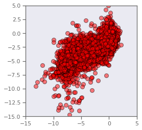
Determine and evaluate the performance of a linear model. You can compare your results with that of the “exact” least-squares result afforded by linear algebra. You may wish to use the LinearRegression model from scikit-learn: https://scikit-learn.org/stable/modules/generated/sklearn.linear_model.LinearRegression.html
# extract data set
y = np.array(soldata.Solubility[:])
X = np.array(soldata[feature_names])
N = len(y)
M = X.shape[1] + 1
A = np.ones((N,M))
A[:,1:] = X[:,:]
#thetaOpt = np.linalg.inv(A.T@A)@A.T@y
thetaOpt = np.linalg.pinv(A)@y
yhat    = A@thetaOpt
fig, ax = plt.subplots()
ax.plot(y,yhat,marker='o',linestyle="",markersize=8,color='r',markeredgecolor='k', alpha = 0.5)
ax.set_aspect('equal', adjustable='box')
plt.xlim(-15,5)
plt.ylim(-15,5)
plt.show()
from sklearn.model_selection  import train_test_split, KFold
from sklearn.linear_model     import LinearRegression, Lasso, Ridge
from sklearn.metrics          import r2_score
from sklearn.preprocessing    import StandardScaler

# We will estimate the model accuracy using cross-validation
y  = np.array(soldata.Solubility[:])
X  = np.array(soldata[feature_names])
k  = 5
kf = KFold(n_splits=k,shuffle=True,random_state=None)
r2 = np.zeros([k])
fig, ax = plt.subplots()
colors =  plt.cm.Accent([i for i in range(k)])
for i,(iTrain,iTest) in enumerate(kf.split(y)):
    Xi_tr = X[iTrain]
    Xi_te = X[iTest]
    yi_tr = y[iTrain]
    yi_te = y[iTest]

    #$$$$$$$$$$$$$$$$$$$$$$$$$$$$$$$$$$$$$$$$$$$$$$$$$$$$$$$$$$
    # perform feature scaling

    # create and test linear regression model

    #$$$$$$$$$$$$$$$$$$$$$$$$$$$$$$$$$$$$$$$$$$$$$$$$$$$$$$$$$$

    r2[i] = r2_score(yi_te,yihat_te)
    ax.plot(yi_te,yihat_te,marker='o',linestyle="",markersize=8,color=colors[i],markeredgecolor='k', alpha = 0.5)
ax.set_aspect('equal', adjustable='box')

print(r2)

plt.xlim(-15,5)
plt.ylim(-15,5)
plt.show()
Regularization
In the previous cells, we considered a model using all possible features, but earlier inspection of the data suggests that some of the features are highly correlated. The implication is that we might obtain a simpler model without any significant loss in accuracy were we to use a different set of features.
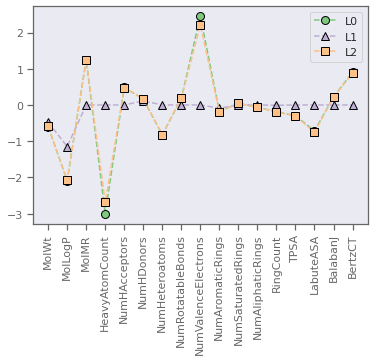
As a first pass towards something akin to feature selection, we will examine the impact of regularization on the model parameters. We discussed L1 and L2 regularization. Use the cells below to examine how using these regularization terms impacts the model parameters (i.e., coefficients). The use of L1 and L2 regularization is sometimes expressed as “Lasso” or “Ridge” regression respectively. There are implementations of these available on scikit-learn:
https://scikit-learn.org/stable/modules/generated/sklearn.linear_model.Lasso.html
https://scikit-learn.org/stable/modules/generated/sklearn.linear_model.Ridge.html
For simplicity, we will just use a simple train/test split. Examine the performance on the test set for the different methods and how this and the produced coefficients are impacted by the regularization weighting.
# set weight for regularization term
my_alpha = 0.2

# create train vs. test split
X_tr, X_te, y_tr, y_te = train_test_split(X,y,test_size = 0.8, random_state = 1)

# feature scaling (here using standard scaling)
scaler = StandardScaler()
scaler.fit(X_tr)
X_tr_sc = scaler.transform(X_tr)

#$$$$$$$$$$$$$$$$$$$$$$$$$$$$$$$$$$$$$$$$$$$$$$$$$$$$$$$$$$
# create and test model with simple linear regression
model_L0  =
yhat_L0   =
r2_L0     =

# create and test model with L1 regularization
model_L1  =
yhat_L1   =
r2_L1     =

# create and test model with L2 regularization
model_L2  =
yhat_L2   =
r2_L2     =
#$$$$$$$$$$$$$$$$$$$$$$$$$$$$$$$$$$$$$$$$$$$$$$$$$$$$$$$$$$


# plot and compare coefficients
fig, ax = plt.subplots()
colors =  plt.cm.Accent([i for i in range(3)])
h      = [0 for i in range(3)]
h[0], = ax.plot(range(M-1),model_L0.coef_,marker='o',linestyle="--",markersize=8,color=colors[0],markeredgecolor='k',label='L0')
h[1], = ax.plot(range(M-1),model_L1.coef_,marker='^',linestyle="--",markersize=8,color=colors[1],markeredgecolor='k',label='L1')
h[2], = ax.plot(range(M-1),model_L2.coef_,marker='s',linestyle="--",markersize=8,color=colors[2],markeredgecolor='k',label='L2')
plt.xticks(range(M-1),feature_names,rotation=90)
ax.legend(handles=h)
plt.show()

print("Coefficients of determination are..")
print("L0: {:>8.3f}, L1: {:>8.3f}, L2: {:>8.3f}".format(r2_L0,r2_L1,r2_L2))
Coefficients of determination are..
L0:    0.468, L1:    0.420, L2:    0.467
Feature Selection
From previous results and analysis, we can probably conclude that we do not need all of the features for an accurate model. We mentioned a variety of feature selection methods. Here, we’ll use a simple greedy correlation filter to remove “redundant” features. Comment the code below between the indicated region to ensure comprehension. How does the result compare to any of the regularization methods? Does this make sense?
#$$$$$$$$$$$$$$$$$$$$$$$$$$$$$$$$$$$$$$$$$$$$$$$$$$$$$$$$$$
rmax        = 0.8
subset      = [n for n in feature_names]
while True:
  absr = np.abs(soldata[subset].corr(method='pearson').to_numpy())
  np.fill_diagonal(absr,0.)
  imax = np.argmax(absr)
  jmax = imax%len(subset)
  imax = int(imax/len(subset))
  if absr[imax,jmax] < rmax:
    break
  rem_n = subset.pop(jmax)
  print("Removing feature {} with correlation of {:>5.3f} with {}".format(rem_n,absr[imax,jmax],subset[imax]))
Xsub = np.array(soldata[subset])
#$$$$$$$$$$$$$$$$$$$$$$$$$$$$$$$$$$$$$$$$$$$$$$$$$$$$$$$$$$


# create train vs. test split
Xsub_tr, Xsub_te, y_tr, y_te = train_test_split(Xsub,y,test_size = 0.8, random_state = 1)

# feature scaling (here using standard scaling)
scaler = StandardScaler()
scaler.fit(Xsub_tr)
Xsub_tr_sc = scaler.transform(Xsub_tr)

# create and test model with simple linear regression
model_L0  = LinearRegression().fit(Xsub_tr_sc, y_tr)
yhat_L0   = model_L0.predict(scaler.transform(Xsub_te))
r2_L0     = r2_score(y_te,yhat_L0)
print(r2_L0)
Activity 3: Fun with Neural Networks
In this activity session, we are going to use the Keras API to build simple, feed-forward deep neural networks. At the end, you will have some freedom to use the API to investigate the impact of hyperparameters and model complexity with the same solubility dataset.
import numpy  as np
import pandas as pd
import tensorflow as tf
from tensorflow       import keras
from tensorflow.keras import layers
from matplotlib import pyplot as plt
import seaborn as sns
from sklearn.preprocessing import StandardScaler
from sklearn.model_selection import KFold
from sklearn.linear_model import LinearRegression,Ridge,Lasso
import sklearn.metrics as sklm
import pydot
import graphviz
Building models with the Sequential API
We will start with the “sequential” model, which is really easy to use! You can play around with the different parameters and check the output with the .summary() method. Can you make sense of the number of parameters that are reported???
# Create Model Container
model = keras.Sequential(name="myFirstModel")

# Define Layers
inputLayer= keras.Input(shape=(4,))
layer1= layers.Dense(10,activation='relu',name="myFirstLayer")
layer2= layers.Dense(8,activation='tanh',name="oldNewsLayer")
output= layers.Dense(1,activation=None,name="outputLayer")

# Add layers to model
model.add(inputLayer)
model.add(layer1)
model.add(layer2)
model.add(output)

# Admire Model
model.summary()
Model: "myFirstModel"
_________________________________________________________________
 Layer (type)                Output Shape              Param #
=================================================================
 myFirstLayer (Dense)        (None, 10)                50

 oldNewsLayer (Dense)        (None, 8)                 88

 outputLayer (Dense)         (None, 1)                 9

=================================================================
Total params: 147
Trainable params: 147
Non-trainable params: 0
_________________________________________________________________
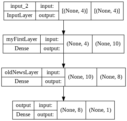
Building models with Functional API
We will also demonstrate the functional API. The functional API is more flexible than the Sequential API and permits you more control over the architecture. By contrast, Sequential models can only be fully connected, feed forward.
# Define Layers
inputLayer = keras.Input(shape=(4,))
layer1= layers.Dense(10,activation='relu',name="myFirstLayer")
layer2= layers.Dense(8,activation='tanh',name="oldNewsLayer")
output= layers.Dense(1,activation=None,name="output")

# Connect layers using "layer calls"
# we want to achieve
# inputLayer --> layer1 --> layer2 --> outputs
x = layer1(inputLayer)
x = layer2(x)
outputs = output(x)

# Build model from inputs/outputs
model = keras.Model(inputs=inputLayer,outputs=outputs,\
        name="mySecondModel")

# Admire Model
model.summary()
keras.utils.plot_model(model,"model.png",show_shapes=True)
Model: "mySecondModel"
_________________________________________________________________
 Layer (type)                Output Shape              Param #
=================================================================
 input_2 (InputLayer)        [(None, 4)]               0

 myFirstLayer (Dense)        (None, 10)                50

 oldNewsLayer (Dense)        (None, 8)                 88

 output (Dense)              (None, 1)                 9

=================================================================
Total params: 147
Trainable params: 147
Non-trainable params: 0
_________________________________________________________________
Return of the Solubility Dataset
So, now we are going to try and apply what we have learned to create a neural network that can predict solubility from chemical descriptors of a molecule. How many features are there to describe each molecule?
# Load and extract the data from dmol-book
soldata = pd.read_csv(
    "https://github.com/whitead/dmol-book/raw/master/data/curated-solubility-dataset.csv"
)
features_start_at = list(soldata.columns).index("MolWt")
feature_names = soldata.columns[features_start_at:]
y = np.array(soldata.Solubility[:]).reshape([-1,1])
X = np.array(soldata[feature_names])
# note the reshape on y above, which forces the structure to a matrix/2d array
# this is the form that will be expected by Keras
# the first index to an array corresponds to a specific example
# the size of the second index is the dimensionality
A deep neural network to predict solubility
Use the cell below to build a neural network to predict solubility from the input features obtained from the .csv. Play around with the architecture to gain some intuition for the predictive capabilities of the network? How small of a network can you make that still yields “good” results (say, \(r^2 > 0.7\))?
inScaler = StandardScaler() # scaler for features
outScaler= StandardScaler() # scaler for labels
inScaler.fit(X)
outScaler.fit(y)
Xsc = inScaler.transform(X)  # these are the scaled features
ysc = outScaler.transform(y) # these are the scaled labels

#$$$$$$$$$$$$$$$$$$$$$$$$$$$$$$$$$$$$$$$$$$$$$$$$$$$$$$$$$$
model  = keras.Sequential() # this initializes our simple model, but it doesn't have anhything in it!
hidden1= layers.Dense(32,activation="relu") # here we create 20-neuron layer with relu activation
hidden2= layers.Dense(5,activation="relu")  # this is a 5-neuron layer, again with relu
out    = layers.Dense(1)    # we will only have one output, activation=None means linear/identity
model.add(hidden1)
model.add(hidden2)
model.add(out)
model.build((None,Xsc.shape[1])) # this last line specifies the input shape; there are lots of ways to do this
model.summary()
#$$$$$$$$$$$$$$$$$$$$$$$$$$$$$$$$$$$$$$$$$$$$$$$$$$$$$$$$$$
keras.utils.plot_model(model,"model.png",show_shapes=True)

# now we compile the model and train it
model.compile(optimizer="SGD",loss="mean_squared_error",metrics=["mean_absolute_error"])
hist = model.fit(x=Xsc,y=ysc,epochs=100,validation_split=0.2)

# make predictions
ypredsc = model.predict(Xsc)
ypred   = outScaler.inverse_transform(ypredsc)
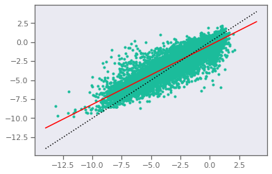
plt.plot(y,ypred,".")
linearFit = LinearRegression().fit(y,ypred)
r2 = sklm.r2_score(y,ypred)
mae= sklm.mean_absolute_error(y,ypred)
mse=sklm.mean_squared_error(y,ypred)
print("r2 = {:>5.2f}, mae = {:>5.2f}, mse = {:>5.2f}".format(r2,mae,mse))
xline = np.array([[-14],[4]])
yline = linearFit.predict(xline)
plt.plot(xline,yline,'-r')
plt.plot(xline,xline,':k')
plt.show()
Model: "sequential_1"
_________________________________________________________________
 Layer (type)                Output Shape              Param #
=================================================================
 dense_3 (Dense)             (None, 32)                576

 dense_4 (Dense)             (None, 5)                 165

 dense_5 (Dense)             (None, 1)                 6

=================================================================
Total params: 747
Trainable params: 747
Non-trainable params: 0
_________________________________________________________________
Epoch 1/100
250/250 [==============================] - 2s 5ms/step - loss: 0.6888 - mean_absolute_error: 0.6227 - val_loss: 0.3194 - val_mean_absolute_error: 0.4420
Epoch 2/100
250/250 [==============================] - 1s 3ms/step - loss: 0.4591 - mean_absolute_error: 0.4895 - val_loss: 0.2744 - val_mean_absolute_error: 0.4052
Epoch 3/100
250/250 [==============================] - 1s 3ms/step - loss: 0.4023 - mean_absolute_error: 0.4559 - val_loss: 0.2615 - val_mean_absolute_error: 0.3947
Epoch 4/100
250/250 [==============================] - 1s 3ms/step - loss: 0.3832 - mean_absolute_error: 0.4442 - val_loss: 0.2518 - val_mean_absolute_error: 0.3878
Epoch 5/100
250/250 [==============================] - 1s 3ms/step - loss: 0.3651 - mean_absolute_error: 0.4332 - val_loss: 0.2546 - val_mean_absolute_error: 0.3903
Epoch 6/100
250/250 [==============================] - 1s 3ms/step - loss: 0.3543 - mean_absolute_error: 0.4258 - val_loss: 0.2511 - val_mean_absolute_error: 0.3867
Epoch 7/100
250/250 [==============================] - 1s 3ms/step - loss: 0.3427 - mean_absolute_error: 0.4195 - val_loss: 0.2425 - val_mean_absolute_error: 0.3780
Epoch 8/100
250/250 [==============================] - 1s 3ms/step - loss: 0.3315 - mean_absolute_error: 0.4119 - val_loss: 0.2406 - val_mean_absolute_error: 0.3760
Epoch 9/100
250/250 [==============================] - 1s 3ms/step - loss: 0.3234 - mean_absolute_error: 0.4072 - val_loss: 0.2512 - val_mean_absolute_error: 0.3821
Epoch 10/100
250/250 [==============================] - 1s 3ms/step - loss: 0.3163 - mean_absolute_error: 0.4018 - val_loss: 0.2447 - val_mean_absolute_error: 0.3793
Epoch 11/100
250/250 [==============================] - 1s 3ms/step - loss: 0.3111 - mean_absolute_error: 0.3991 - val_loss: 0.2480 - val_mean_absolute_error: 0.3801
Epoch 12/100
250/250 [==============================] - 1s 3ms/step - loss: 0.3065 - mean_absolute_error: 0.3962 - val_loss: 0.2418 - val_mean_absolute_error: 0.3780
Epoch 13/100
250/250 [==============================] - 1s 4ms/step - loss: 0.3019 - mean_absolute_error: 0.3921 - val_loss: 0.2411 - val_mean_absolute_error: 0.3765
Epoch 14/100
250/250 [==============================] - 1s 3ms/step - loss: 0.2986 - mean_absolute_error: 0.3902 - val_loss: 0.2343 - val_mean_absolute_error: 0.3752
Epoch 15/100
250/250 [==============================] - 0s 2ms/step - loss: 0.2956 - mean_absolute_error: 0.3881 - val_loss: 0.2273 - val_mean_absolute_error: 0.3652
Epoch 16/100
250/250 [==============================] - 0s 2ms/step - loss: 0.2917 - mean_absolute_error: 0.3857 - val_loss: 0.2302 - val_mean_absolute_error: 0.3698
Epoch 17/100
250/250 [==============================] - 0s 2ms/step - loss: 0.2887 - mean_absolute_error: 0.3834 - val_loss: 0.2319 - val_mean_absolute_error: 0.3640
Epoch 18/100
250/250 [==============================] - 0s 2ms/step - loss: 0.2879 - mean_absolute_error: 0.3842 - val_loss: 0.2425 - val_mean_absolute_error: 0.3774
Epoch 19/100
250/250 [==============================] - 1s 2ms/step - loss: 0.2877 - mean_absolute_error: 0.3835 - val_loss: 0.2364 - val_mean_absolute_error: 0.3711
Epoch 20/100
250/250 [==============================] - 0s 2ms/step - loss: 0.2837 - mean_absolute_error: 0.3805 - val_loss: 0.2343 - val_mean_absolute_error: 0.3721
Epoch 21/100
250/250 [==============================] - 0s 2ms/step - loss: 0.2817 - mean_absolute_error: 0.3792 - val_loss: 0.2420 - val_mean_absolute_error: 0.3781
Epoch 22/100
250/250 [==============================] - 0s 2ms/step - loss: 0.2810 - mean_absolute_error: 0.3795 - val_loss: 0.2298 - val_mean_absolute_error: 0.3682
Epoch 23/100
250/250 [==============================] - 1s 2ms/step - loss: 0.2786 - mean_absolute_error: 0.3768 - val_loss: 0.2275 - val_mean_absolute_error: 0.3681
Epoch 24/100
250/250 [==============================] - 0s 2ms/step - loss: 0.2778 - mean_absolute_error: 0.3761 - val_loss: 0.2148 - val_mean_absolute_error: 0.3563
Epoch 25/100
250/250 [==============================] - 0s 2ms/step - loss: 0.2762 - mean_absolute_error: 0.3745 - val_loss: 0.2274 - val_mean_absolute_error: 0.3655
Epoch 26/100
250/250 [==============================] - 0s 2ms/step - loss: 0.2748 - mean_absolute_error: 0.3736 - val_loss: 0.2214 - val_mean_absolute_error: 0.3608
Epoch 27/100
250/250 [==============================] - 0s 2ms/step - loss: 0.2723 - mean_absolute_error: 0.3730 - val_loss: 0.2293 - val_mean_absolute_error: 0.3691
Epoch 28/100
250/250 [==============================] - 0s 2ms/step - loss: 0.2713 - mean_absolute_error: 0.3725 - val_loss: 0.2239 - val_mean_absolute_error: 0.3608
Epoch 29/100
250/250 [==============================] - 0s 2ms/step - loss: 0.2702 - mean_absolute_error: 0.3708 - val_loss: 0.2352 - val_mean_absolute_error: 0.3703
Epoch 30/100
250/250 [==============================] - 0s 2ms/step - loss: 0.2697 - mean_absolute_error: 0.3704 - val_loss: 0.2387 - val_mean_absolute_error: 0.3741
Epoch 31/100
250/250 [==============================] - 0s 2ms/step - loss: 0.2680 - mean_absolute_error: 0.3679 - val_loss: 0.2083 - val_mean_absolute_error: 0.3495
Epoch 32/100
250/250 [==============================] - 0s 2ms/step - loss: 0.2684 - mean_absolute_error: 0.3703 - val_loss: 0.2209 - val_mean_absolute_error: 0.3587
Epoch 33/100
250/250 [==============================] - 0s 2ms/step - loss: 0.2678 - mean_absolute_error: 0.3697 - val_loss: 0.2253 - val_mean_absolute_error: 0.3642
Epoch 34/100
250/250 [==============================] - 0s 2ms/step - loss: 0.2668 - mean_absolute_error: 0.3682 - val_loss: 0.2241 - val_mean_absolute_error: 0.3660
Epoch 35/100
250/250 [==============================] - 0s 2ms/step - loss: 0.2652 - mean_absolute_error: 0.3677 - val_loss: 0.2162 - val_mean_absolute_error: 0.3554
Epoch 36/100
250/250 [==============================] - 0s 2ms/step - loss: 0.2663 - mean_absolute_error: 0.3674 - val_loss: 0.2280 - val_mean_absolute_error: 0.3647
Epoch 37/100
250/250 [==============================] - 0s 2ms/step - loss: 0.2637 - mean_absolute_error: 0.3669 - val_loss: 0.2195 - val_mean_absolute_error: 0.3579
Epoch 38/100
250/250 [==============================] - 0s 2ms/step - loss: 0.2627 - mean_absolute_error: 0.3661 - val_loss: 0.2368 - val_mean_absolute_error: 0.3739
Epoch 39/100
250/250 [==============================] - 1s 2ms/step - loss: 0.2628 - mean_absolute_error: 0.3652 - val_loss: 0.2157 - val_mean_absolute_error: 0.3548
Epoch 40/100
250/250 [==============================] - 0s 2ms/step - loss: 0.2626 - mean_absolute_error: 0.3649 - val_loss: 0.2319 - val_mean_absolute_error: 0.3674
Epoch 41/100
250/250 [==============================] - 0s 2ms/step - loss: 0.2615 - mean_absolute_error: 0.3653 - val_loss: 0.2284 - val_mean_absolute_error: 0.3626
Epoch 42/100
250/250 [==============================] - 0s 2ms/step - loss: 0.2590 - mean_absolute_error: 0.3622 - val_loss: 0.2233 - val_mean_absolute_error: 0.3602
Epoch 43/100
250/250 [==============================] - 0s 2ms/step - loss: 0.2602 - mean_absolute_error: 0.3627 - val_loss: 0.2642 - val_mean_absolute_error: 0.3834
Epoch 44/100
250/250 [==============================] - 0s 2ms/step - loss: 0.2590 - mean_absolute_error: 0.3621 - val_loss: 0.2121 - val_mean_absolute_error: 0.3512
Epoch 45/100
250/250 [==============================] - 0s 2ms/step - loss: 0.2590 - mean_absolute_error: 0.3635 - val_loss: 0.2398 - val_mean_absolute_error: 0.3697
Epoch 46/100
250/250 [==============================] - 0s 2ms/step - loss: 0.2578 - mean_absolute_error: 0.3626 - val_loss: 0.2449 - val_mean_absolute_error: 0.3775
Epoch 47/100
250/250 [==============================] - 0s 2ms/step - loss: 0.2573 - mean_absolute_error: 0.3620 - val_loss: 0.2142 - val_mean_absolute_error: 0.3531
Epoch 48/100
250/250 [==============================] - 0s 2ms/step - loss: 0.2552 - mean_absolute_error: 0.3607 - val_loss: 0.2240 - val_mean_absolute_error: 0.3602
Epoch 49/100
250/250 [==============================] - 1s 2ms/step - loss: 0.2556 - mean_absolute_error: 0.3610 - val_loss: 0.2705 - val_mean_absolute_error: 0.3960
Epoch 50/100
250/250 [==============================] - 0s 2ms/step - loss: 0.2567 - mean_absolute_error: 0.3612 - val_loss: 0.2111 - val_mean_absolute_error: 0.3514
Epoch 51/100
250/250 [==============================] - 1s 2ms/step - loss: 0.2557 - mean_absolute_error: 0.3602 - val_loss: 0.2363 - val_mean_absolute_error: 0.3672
Epoch 52/100
250/250 [==============================] - 1s 2ms/step - loss: 0.2565 - mean_absolute_error: 0.3612 - val_loss: 0.2318 - val_mean_absolute_error: 0.3637
Epoch 53/100
250/250 [==============================] - 0s 2ms/step - loss: 0.2537 - mean_absolute_error: 0.3584 - val_loss: 0.2191 - val_mean_absolute_error: 0.3551
Epoch 54/100
250/250 [==============================] - 0s 2ms/step - loss: 0.2534 - mean_absolute_error: 0.3588 - val_loss: 0.2344 - val_mean_absolute_error: 0.3685
Epoch 55/100
250/250 [==============================] - 0s 2ms/step - loss: 0.2515 - mean_absolute_error: 0.3576 - val_loss: 0.2470 - val_mean_absolute_error: 0.3808
Epoch 56/100
250/250 [==============================] - 0s 2ms/step - loss: 0.2530 - mean_absolute_error: 0.3589 - val_loss: 0.2216 - val_mean_absolute_error: 0.3572
Epoch 57/100
250/250 [==============================] - 0s 2ms/step - loss: 0.2501 - mean_absolute_error: 0.3565 - val_loss: 0.2210 - val_mean_absolute_error: 0.3573
Epoch 58/100
250/250 [==============================] - 1s 2ms/step - loss: 0.2505 - mean_absolute_error: 0.3562 - val_loss: 0.2217 - val_mean_absolute_error: 0.3583
Epoch 59/100
250/250 [==============================] - 0s 2ms/step - loss: 0.2509 - mean_absolute_error: 0.3570 - val_loss: 0.2056 - val_mean_absolute_error: 0.3445
Epoch 60/100
250/250 [==============================] - 0s 2ms/step - loss: 0.2502 - mean_absolute_error: 0.3578 - val_loss: 0.2376 - val_mean_absolute_error: 0.3720
Epoch 61/100
250/250 [==============================] - 0s 2ms/step - loss: 0.2507 - mean_absolute_error: 0.3574 - val_loss: 0.2092 - val_mean_absolute_error: 0.3479
Epoch 62/100
250/250 [==============================] - 1s 2ms/step - loss: 0.2482 - mean_absolute_error: 0.3552 - val_loss: 0.2179 - val_mean_absolute_error: 0.3542
Epoch 63/100
250/250 [==============================] - 0s 2ms/step - loss: 0.2484 - mean_absolute_error: 0.3574 - val_loss: 0.2214 - val_mean_absolute_error: 0.3565
Epoch 64/100
250/250 [==============================] - 0s 2ms/step - loss: 0.2492 - mean_absolute_error: 0.3550 - val_loss: 0.2079 - val_mean_absolute_error: 0.3474
Epoch 65/100
250/250 [==============================] - 0s 2ms/step - loss: 0.2469 - mean_absolute_error: 0.3538 - val_loss: 0.2325 - val_mean_absolute_error: 0.3698
Epoch 66/100
250/250 [==============================] - 0s 2ms/step - loss: 0.2469 - mean_absolute_error: 0.3541 - val_loss: 0.2408 - val_mean_absolute_error: 0.3778
Epoch 67/100
250/250 [==============================] - 0s 2ms/step - loss: 0.2483 - mean_absolute_error: 0.3550 - val_loss: 0.2317 - val_mean_absolute_error: 0.3675
Epoch 68/100
250/250 [==============================] - 0s 2ms/step - loss: 0.2459 - mean_absolute_error: 0.3528 - val_loss: 0.2124 - val_mean_absolute_error: 0.3504
Epoch 69/100
250/250 [==============================] - 0s 2ms/step - loss: 0.2463 - mean_absolute_error: 0.3541 - val_loss: 0.2116 - val_mean_absolute_error: 0.3495
Epoch 70/100
250/250 [==============================] - 0s 2ms/step - loss: 0.2467 - mean_absolute_error: 0.3535 - val_loss: 0.2291 - val_mean_absolute_error: 0.3637
Epoch 71/100
250/250 [==============================] - 0s 2ms/step - loss: 0.2459 - mean_absolute_error: 0.3525 - val_loss: 0.2089 - val_mean_absolute_error: 0.3474
Epoch 72/100
250/250 [==============================] - 0s 2ms/step - loss: 0.2437 - mean_absolute_error: 0.3524 - val_loss: 0.2181 - val_mean_absolute_error: 0.3551
Epoch 73/100
250/250 [==============================] - 0s 2ms/step - loss: 0.2451 - mean_absolute_error: 0.3529 - val_loss: 0.2238 - val_mean_absolute_error: 0.3583
Epoch 74/100
250/250 [==============================] - 0s 2ms/step - loss: 0.2475 - mean_absolute_error: 0.3540 - val_loss: 0.2638 - val_mean_absolute_error: 0.3934
Epoch 75/100
250/250 [==============================] - 0s 2ms/step - loss: 0.2440 - mean_absolute_error: 0.3532 - val_loss: 0.2195 - val_mean_absolute_error: 0.3589
Epoch 76/100
250/250 [==============================] - 0s 2ms/step - loss: 0.2427 - mean_absolute_error: 0.3518 - val_loss: 0.2029 - val_mean_absolute_error: 0.3423
Epoch 77/100
250/250 [==============================] - 0s 2ms/step - loss: 0.2430 - mean_absolute_error: 0.3528 - val_loss: 0.2221 - val_mean_absolute_error: 0.3564
Epoch 78/100
250/250 [==============================] - 0s 2ms/step - loss: 0.2439 - mean_absolute_error: 0.3535 - val_loss: 0.2201 - val_mean_absolute_error: 0.3561
Epoch 79/100
250/250 [==============================] - 0s 2ms/step - loss: 0.2435 - mean_absolute_error: 0.3525 - val_loss: 0.2442 - val_mean_absolute_error: 0.3725
Epoch 80/100
250/250 [==============================] - 1s 2ms/step - loss: 0.2414 - mean_absolute_error: 0.3512 - val_loss: 0.2167 - val_mean_absolute_error: 0.3525
Epoch 81/100
250/250 [==============================] - 0s 2ms/step - loss: 0.2421 - mean_absolute_error: 0.3517 - val_loss: 0.2300 - val_mean_absolute_error: 0.3627
Epoch 82/100
250/250 [==============================] - 1s 2ms/step - loss: 0.2412 - mean_absolute_error: 0.3508 - val_loss: 0.2063 - val_mean_absolute_error: 0.3461
Epoch 83/100
250/250 [==============================] - 0s 2ms/step - loss: 0.2421 - mean_absolute_error: 0.3503 - val_loss: 0.2063 - val_mean_absolute_error: 0.3453
Epoch 84/100
250/250 [==============================] - 0s 2ms/step - loss: 0.2412 - mean_absolute_error: 0.3510 - val_loss: 0.2233 - val_mean_absolute_error: 0.3578
Epoch 85/100
250/250 [==============================] - 0s 2ms/step - loss: 0.2394 - mean_absolute_error: 0.3498 - val_loss: 0.2138 - val_mean_absolute_error: 0.3540
Epoch 86/100
250/250 [==============================] - 0s 2ms/step - loss: 0.2419 - mean_absolute_error: 0.3512 - val_loss: 0.2221 - val_mean_absolute_error: 0.3574
Epoch 87/100
250/250 [==============================] - 1s 2ms/step - loss: 0.2406 - mean_absolute_error: 0.3495 - val_loss: 0.2574 - val_mean_absolute_error: 0.3823
Epoch 88/100
250/250 [==============================] - 0s 2ms/step - loss: 0.2388 - mean_absolute_error: 0.3502 - val_loss: 0.2185 - val_mean_absolute_error: 0.3538
Epoch 89/100
250/250 [==============================] - 0s 2ms/step - loss: 0.2400 - mean_absolute_error: 0.3495 - val_loss: 0.2208 - val_mean_absolute_error: 0.3569
Epoch 90/100
250/250 [==============================] - 0s 2ms/step - loss: 0.2387 - mean_absolute_error: 0.3501 - val_loss: 0.2077 - val_mean_absolute_error: 0.3466
Epoch 91/100
250/250 [==============================] - 0s 2ms/step - loss: 0.2393 - mean_absolute_error: 0.3490 - val_loss: 0.2122 - val_mean_absolute_error: 0.3505
Epoch 92/100
250/250 [==============================] - 1s 2ms/step - loss: 0.2385 - mean_absolute_error: 0.3492 - val_loss: 0.2171 - val_mean_absolute_error: 0.3542
Epoch 93/100
250/250 [==============================] - 1s 2ms/step - loss: 0.2377 - mean_absolute_error: 0.3477 - val_loss: 0.2249 - val_mean_absolute_error: 0.3613
Epoch 94/100
250/250 [==============================] - 0s 2ms/step - loss: 0.2381 - mean_absolute_error: 0.3479 - val_loss: 0.2125 - val_mean_absolute_error: 0.3528
Epoch 95/100
250/250 [==============================] - 0s 2ms/step - loss: 0.2380 - mean_absolute_error: 0.3480 - val_loss: 0.2355 - val_mean_absolute_error: 0.3675
Epoch 96/100
250/250 [==============================] - 0s 2ms/step - loss: 0.2377 - mean_absolute_error: 0.3478 - val_loss: 0.2206 - val_mean_absolute_error: 0.3556
Epoch 97/100
250/250 [==============================] - 0s 2ms/step - loss: 0.2371 - mean_absolute_error: 0.3471 - val_loss: 0.2095 - val_mean_absolute_error: 0.3482
Epoch 98/100
250/250 [==============================] - 0s 2ms/step - loss: 0.2364 - mean_absolute_error: 0.3472 - val_loss: 0.2112 - val_mean_absolute_error: 0.3484
Epoch 99/100
250/250 [==============================] - 0s 2ms/step - loss: 0.2374 - mean_absolute_error: 0.3478 - val_loss: 0.2249 - val_mean_absolute_error: 0.3636
Epoch 100/100
250/250 [==============================] - 0s 2ms/step - loss: 0.2362 - mean_absolute_error: 0.3469 - val_loss: 0.2171 - val_mean_absolute_error: 0.3577
r2 =  0.76, mae =  0.85, mse =  1.35
[<matplotlib.lines.Line2D at 0x7fc5b550cc10>]
Learning curves
We can monitor the history of training and inspect it to get a sense of convergence/underfitting/overfitting during optimization. Do you think the current model is overfit?
print(hist.history.keys())
loss = hist.history['loss']
val_loss = hist.history['val_loss']
plt.plot(loss,'-k')
plt.plot(val_loss,':r')
plt.show()